Solving for work/life balance

Preface

This was a for-fun thought experiment that I did years ago at the beginning of the pandemic when we were all isolating.

Motivation

It’s April 2020 and the world has come to a grinding halt with Covid-19. In hindsight, I think we saw this coming (I’m looking back at SARS and MERS). The silver lining of this tragedy–in my humble opinion–is how open scientists and physicians are at sharing what they learn and how the community as a whole is working together to come up with a solution – at least for the moment. Covid-19 is not the main subject of this post, per se, because there are plenty of other researchers doing great science. So what am I going to talk about? Well, this pandemic actually brings up something that is affecting a lot of us: work/life balance.

One of the most effective things we have in our tiny arsenal against spreading SARS-CoV-2 is social isolation so, those who can, are working from home. Here, the balance of work pressures and life pressures has been off-kilter. Normally, working from home for me is a mix of working at my little home office or the corner coffee shop or library by my house. In either case, kids are not a problem because of the nanny and school. But in April 2020, the schools are closed, the library is closed, the nanny is quarantined following an ER visit (unrelated), and I honestly don’t think that coffee shop will ever reopen after this hit. Yikes!

Life is, of course, stochastic. There are many different factors at play and some are just random or dumb luck. Nevertheless, I thought it would be a fun exercise to model how one’s wellbeing can positively contribute to work and how work, in turn, might influence someone’s wellbeing (e.g., a paycheck, contributing to a worthy cause). However, there is only so much work that one can do before it starts to affect life.

So there’s feedback here but how exactly work and life feed into each other seem to be different for every person. For example, do you know some people who seem to roll with every punch? Little disturbances seem to just bounce off them and the quickly find themselves right back at their steady-state. For others, disturbances can really throw off things and they find themselves spiraling and having trouble balancing between different work and life pressures under a fixed time interval.

While this is a fun exercise I did while sitting at home under the stay-at-home order, my hope is that this model might train some intuition about bouncing back from big work or life events. So here we go.

The model

Let’s consider \(x\) to be proportional to one’s wellbeing and let \(y\) be proportional to their work productivity. A system of differential equations for the change of \(x\) and \(y\) across time might look like this:

\[ \begin{matrix} \frac{dx}{dt}= x (1 - \frac{x}{K}) - \frac{x y}{x + \theta} \\ \frac{dy}{dt}= \frac{x y}{x + \theta} - \frac{1}{4} y \end{matrix} \]

where \(K\) is the maximum level of wellbeing. This level is set by the individual and ties in all of the “needs” to achieve their desired wellbeing. Needs could include material things, home size, and proximity to shops, etc. The parameter \(\theta\) is related to the intensity of work pressure. Note that the interaction term that contains \(\theta\) is the functional response and depends on wellbeing as well as current levels of work productivity. To see how this interaction behaves, take a look at the plot below where the work productivity is held constant (at 100) and both wellbeing and \(\theta\) vary.

x <- seq(from=0, to=200, by=0.01)
y <- 100
theta <- seq(from=10, to=210, by=20)

dat <- expand.grid(x=x, y=y, theta=theta)

dat$response <- apply(dat, 1, function(a){
  x = a[1] # explicitly labeled here for readability
  y = a[2]
  theta = a[3]
  return((-x*y)/(x+theta))
})
dat$theta <- as.factor(dat$theta)

ggplot(data=dat, aes(x=x, y=response, group=theta)) +
     geom_line(aes(colour=theta)) +
     theme_light() +
     ylab("Change in wellbeing from the interaction term") +
     xlab("Wellbeing (X) when holding Y to 100")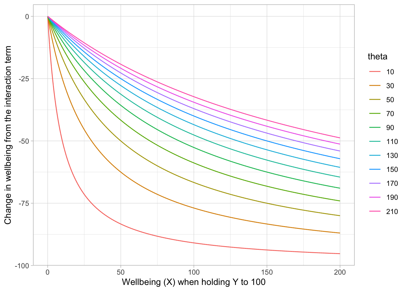

You can see that small values of \(\theta\) translate to a large response (greater negative) for any given value of wellbeing. In other words, if both wellbeing and \(\theta\) are small, the response is large and negative compared to cases where either wellbeing or \(\theta\) are larger. Setting smaller values of \(y\) does not change the relative shape of these different curves but does change the absolute magnitude–the y-axis scale–of change since it’s present in the numerator (data not shown).

In this model, the instantaneous change in work productivity, \(\frac{dy}{dt}\), is positively affected by this interaction term. And in the absence of any wellbeing, I arbitrarily set the model to decrease the productivity amount by a quarter.

Model behavior

Okay, so how does this model behave? Let’s first look at the x- and y-isoclines. The equilibria values are where any x-isocline intersects with any y-isocline (but we can also solve for these equilibria directly). The isoclines are determined by setting the respective equations to zero and solving.

For the x-isoclines, the solutions are \(x=0\) and \(y=\frac{(K-x)(\theta+x)}{K}\). The first is just a vertical line and the second is a curve that resembles this:

x <- seq(from=0, to=35, by=0.01)
theta <- 10
k <- 30
fofx <- function(x, k, theta){
     return(((k-x)*(theta+x))/k)
}

plot(x, fofx(x=x, k=k, theta=theta), ylab="Work Productivity", xlab="Wellbeing", type="l", lty="dotdash", col="red", xlim=c(0, 35), ylim=c(0, 20), main=expression(paste("x-isoclines; ", plain(theta), "=10  and  ",plain(K), "=30")))
abline(v=0, lty="dotdash", col="red")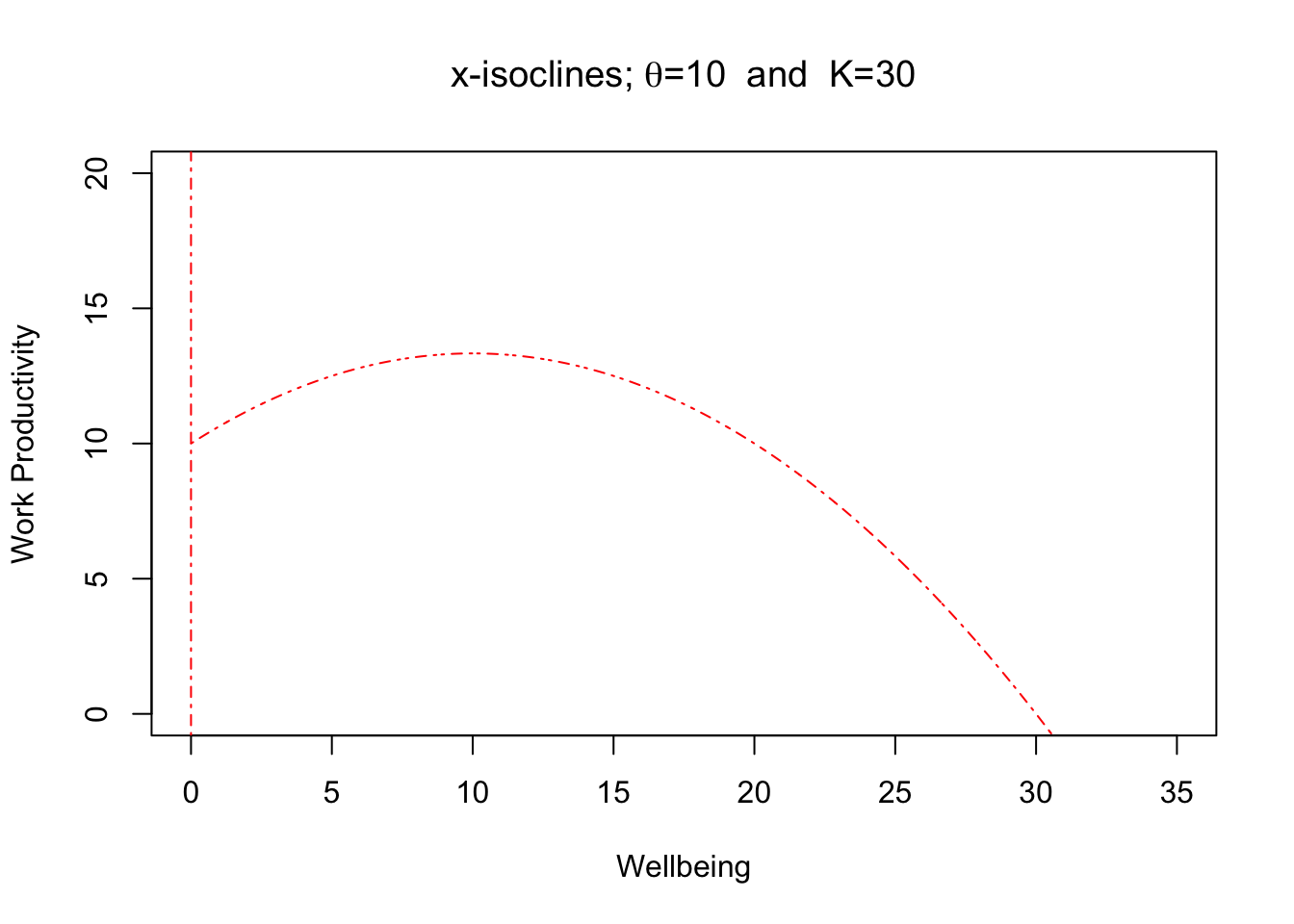

These are locations where the work/life balance trajectories only go into the vertical position (up and down).

For the y-isoclines, we get one horizontal line (\(y=0\)) and one vertical line (\(x=\frac{\theta}{3}\)). These are the locations where work/life trajectories only go into the horizontal position (left and right).

plot(x=NULL, y=NULL, xlim=c(0, 35), ylim=c(0, 20), 
     ylab="Work Productivity", xlab="Wellbeing",  
     main=expression(paste("y-isoclines; ", plain(theta), "=10")))
abline(v=theta/3, lty="dashed", col="blue")
abline(h=0, lty="dashed", col="blue")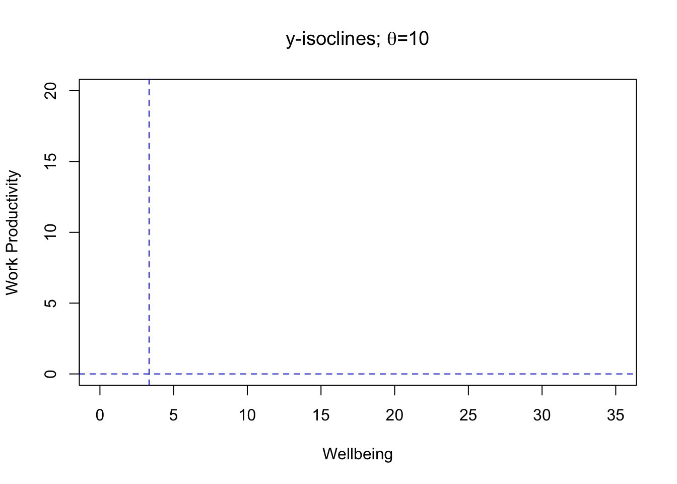

And putting these all together and picking some values of \(\theta\) (10) and \(K\) (30), we get all the isoclines:

x <- seq(from=0, to=35, by=0.01)
theta <- 10
k <- 30
fofx <- function(x, k, theta){
     return(((k-x)*(theta+x))/k)
}

plot(x, fofx(x=x, k=k, theta=theta), ylab="Work Productivity", 
     xlab="Wellbeing", type="l", lty="dotdash", col="red", xlim=c(0, 35), 
     ylim=c(0, 20), main="x-isoclines (red) and y-isoclines (blue)")
abline(v=0, lty="dotdash", col="red")
abline(v=theta/3, lty="dashed", col="blue")
abline(h=0, lty="dashed", col="blue")
points(x=theta/3, y=fofx(x=theta/3, k=30, theta=theta)) # Interior equalibirum
points(x=0,y=0)
points(x=k, y=0)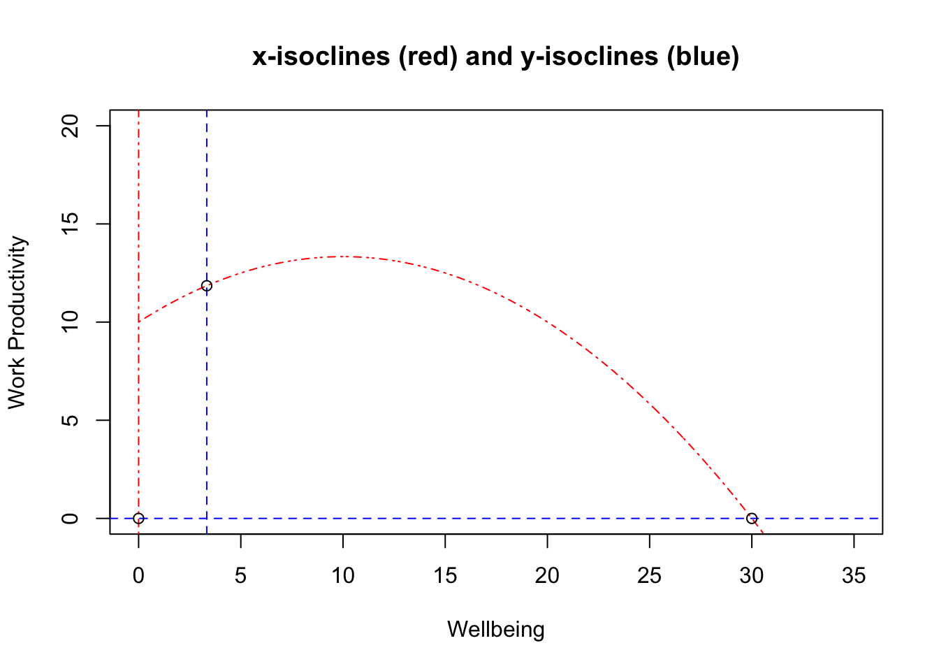

So there are (up to) three equilibria (i.e., up to one internal equilibrium). Each line segment above has either 1) an up or down (red) or 2) a left or right (blue) direction. Looking at the change along each segment can reveal the direction. For example, for the y-isocline \(y=0\), we can evaluate the instantaneous change of the wellbeing equation at various points along that line: \[\frac{dx}{dt} \bigg\rvert_{y = 0 } = x (1 - \frac{x}{K})\]

Here, \(x\) is either 0 (which would be an equilibrium point [x=0,y=0]) or positive so we only need to consider the sign of what is in the parentheses. Inside the parentheses, the expression is negative (left direction) when \(x>K\) and is positive (right arrow) when \(x<K\). This should make sense: in the absence of \(y\), \(\frac{dx}{dt}\) behaves just like a logistic equation and reaches an equilibrium value of \(K\). We know from the logistic that \(K\) is a stable equilibrium: any perturbations from it (in only the one-dimensional case, that is), will have \(x\) bounce back to \(K\), eventually. The stability of the two-dimensional case need not be stable since perturbations can occur in the y direction.

Stablility

To look at stablility, let’s take a look at the Jacobian matrix of this model:

\[J(x,y) = \begin{bmatrix} \frac{\partial f_1}{\partial x} & \frac{\partial f_1}{\partial y} \\ \frac{\partial f_2}{\partial x} & \frac{\partial f_2}{\partial y} \end{bmatrix} = \begin{bmatrix} -\frac{2 x}{K} - \frac{\theta y}{(\theta + x)^2} + 1 & -\frac{x}{\theta + x}\\ \frac{\theta y}{(\theta + x)^2} & \frac{x}{\theta + x} - \frac{1}{4} \end{bmatrix}\].

The block below defines some functions that can help us numerically solve individual components of the Jacobian.

aa <- function(x, y, theta, K){
     return(-((2*x)/(K)) - ((theta * y)/(theta + x)^2) + 1)
}
bb <- function(x, y, theta, K){
     return(-x/(theta + x))
}
cc <- function(x, y, theta, K){
     return((theta * y)/(theta + x)^2)
}
dd <- function(x, y, theta, K){
     return(((x)/(theta + x)) - (1/4))
}

trace <- function(x, y, theta, K){
     return(aa(x, y, theta, K)+dd(x, y, theta, K))
}
det <- function(x, y, theta, K){
  out <- aa(x, y, theta, K)*dd(x, y, theta, K) - bb(x, y, theta, K)*cc(x, y, theta, K)
     return(out)
}

So for point [x=30, y=0] mentioned above with parameters \(\theta=10\) and \(K=30\), \[J(30,0) = \begin{bmatrix} -1 & -\frac{3}{4} \\ 0 & \frac{1}{2} \end{bmatrix}\]

The trace of this is negative (\(\beta=-\frac{1}{2}\)) but the determinate is also negative (\(\gamma=-\frac{1}{2}\)); thus, the equalibrium point [30,0] is not stable for this model and for these parameters (it’s a saddle).

Let’s take a look at that interior equilibrium [\(x=\frac{\theta}{3}\), \(y \cong 11.85185\)]. Here, both the trace and determinate are positive:

# trace
beta <- trace(x=theta/3, y=fofx(x=theta/3, k=k, theta=theta), theta, k) # y = 11.85185
beta

[1] 0.1111111

# determinate
gamma <- det(x=theta/3, y=fofx(x=theta/3, k=k, theta=theta), theta, k)
gamma

[1] 0.1666667

Can we learn anything else? We can take a look at the eigenvalues to determine if there are any complex parts (which would be indicative of oscillations).

\[ \lambda_1, \lambda_2 = \frac{\beta \pm \sqrt[]{\beta^2 - 4 \gamma}}{2} \]

Here we can see there is an imaginary part (negative in the square root). So there’s evidence of oscillations.

beta^2 - 4*gamma

[1] -0.654321

Visualizing trajectories in R

Let’s visualize what happens to one’s work/life balance when they start at some point (\(x>0\), \(y>0\)) with some fixed pair of parameters. For this part, we’ll use the R package deSolve. But first, let’s define a plotting function to visualize trajectories using R’s ggplot2.

plot_df <- function(DF, params){
     require(ggplot2)
     require(dplyr)

     x <- seq(from=0, to=max(DF$X*1.5), length.out=200)
     y <- ((parms["K"]-x)*(parms["theta"]+x))/(parms["K"])
     df2 <- data.frame(x=x, y=y) %>% filter(y>=0, x>=0)

     p <- ggplot(data=DF, aes(x= X, y=Y)) +
          geom_path(arrow = arrow(type = "open", angle = 30, length = unit(0.1, "inches"))) +
          theme_light() +
          xlab("Wellbeing") + ylab("Work Productivity") +
          scale_x_continuous(limits=c(0, max(c(max(1.2*x), max(1.2*DF["X"]))))) +
          scale_y_continuous(limits=c(0, max(c(max(1.2*y), max(1.2*DF["Y"])))))

     p <- p + geom_path(data=df2, aes(x=x,y=y), colour="red", linetype="dotdash")
     p <- p + geom_vline(xintercept = 0, colour="red", linetype="dotdash")

     p <- p + geom_vline(xintercept = parms["theta"]/3, colour="blue", linetype='dashed')
     p <- p + geom_hline(yintercept = 0, colour="blue", linetype='dashed')

     return(p)
}

System of ODEs can be written like this:

model <- function(t, y, parms){
     with(as.list(c(y, parms)), {
          # y[1] is X and y[2] is Y
          dX <- y[1] * (1 - (y[1]/K)) - (y[1]*y[2])/(y[1]+theta)
          dY <- -0.25*y[2] + (y[1]*y[2])/(y[1]+theta)
          list(c(dX, dY))
     })
}

Let’s take a look at our parameters that we’ve been working with and start the initial \(x\),\(y\) coordinates to [10,10].

parms <- c(K = 30, theta=10)
yini <- c(X = 10, Y=10)
times <- seq(0, 1000, 1)
out <- ode(times=times, y = yini, func = model, parms=parms)

#diagnostics(out)
df <- as.data.frame(out)

plot_df(df)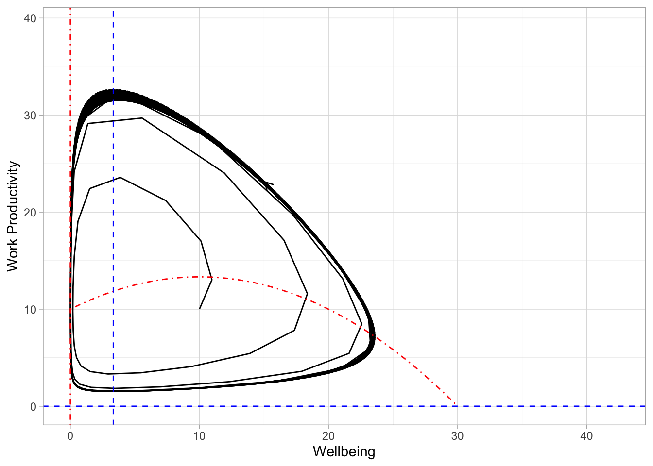

In the plot above, we can see that the formation of a periodic orbit: starting at point [10,10] and following 1000 time steps (the last step is where the arrowhead occurs). With this example, \(\theta\) was very small and so it makes sense that small changes in work productivity have large changes in wellbeing in this model. Under these conditions, large swings between wellbeing and work productivity occur.

Let’s take a look at another condition: when \(\theta\) is larger.

parms <- c(K = 30, theta=30)
yini <- c(X = 10, Y=10)
times <- seq(0, 1000, 1)
out <- ode(times=times, y = yini, func = model, parms=parms)

#diagnostics(out)
df <- as.data.frame(out)

plot_df(df)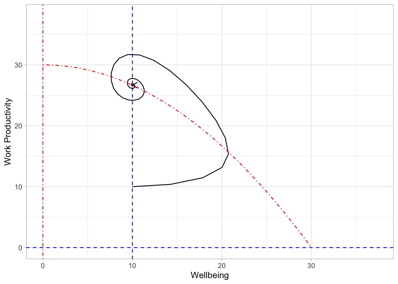

When \(\theta=30\), we get a spiral towards the equilibrium! We can see that \(\beta < 0\) and that \(\gamma > 0\) so we have stability plus there’s an imaginary part of the eigenvalues so there are oscillations towards this equilibrium.

beta1 <- trace(x=30/3, y=fofx(x=30/3, k=30, theta=30), theta=30, K = 30)
beta1

[1] -0.1666667

gamma1 <- det(x=30/3, y=fofx(x=30/3, k=30, theta=30), theta=30, K = 30)
gamma1

[1] 0.125

beta1^2 - 4*gamma1

[1] -0.4722222

This result is analogous to that zen coworker you know. In this situation, some event occurred that knocked them off their internal equilibrium by decreasing work productivity. Following that event, their wellbeing increased which, in turn, allowed their work productivity to also increase. That increase to some maximum and then there was a back and forth. Importantly, that back and forth is continually dampened until reaching an equilibrium. Keep in mind that actually reaching the equilibrium wasn’t the point here. The b_ehavior_ of dampening down work/life towards a steady-state was one of the things I was looking for in a work/life balance model.

A deeper dive

So how do we get some cases where there are orbits and other cases where there are spiraling back towards an equilibrium?

If you look at that x-isocline that curves, you can see a difference between the above two plots above. The y-isocline \[\frac{\theta}{3}\] is located on the incline of the curve in the first plot but is on the decline of the curve on the second plot. Let’s take a deeper look to see if the y-isocline position can tell us the trajectory behavior.

Taking the derivitative of the curved x-isocline we can identify the maximum point. So the x-isocline is:

\[y = \frac{(K-x)(\theta + x)}{K}\]

and the derivative is:

\[y' = \frac{K-\theta - 2 x}{K}\]

Setting \(y'\) to zero and solving for \(x\) yields:

\[x = \frac{K-\theta}{2}\]

So there are three conditions:

1. The y-isocline \(\frac{\theta}{3}\) is on the positive slope when \(\frac{\theta}{3} < \frac{K-\theta}{2} \Rightarrow K > \frac{5}{3}\theta\) and

2. is on the negative slope when \(\frac{\theta}{3} > \frac{K-\theta}{2} \Rightarrow K < \frac{5}{3}\theta\) and

3. zero slope when \(K = \frac{5}{3}\theta\)

So what does this model tell us?

By now you should now that this is just a model and doesn’t necessarily reflect real, stochastic life. That being said, there’s one thing I wanted a model to capture. That is, why some individuals seem to bounce right back from minor perturbations while others seem to be in a constant struggle with work and life vying for their time.

How to achieve zen-like work/life balance? From this model, either 1) reducing the set point of your wellbeing (i.e., being happy with less) or 2) reduce the degree to which work pressures affect your wellbeing or 3) a combination of 1 and 2 are key. Those are no small changes and I recommend the reader to work/life balance books for instruction.

Equations weren’t necessary to say that happier individuals are more productive, of course. Having good work/life balance depends on 1) the set of things that make one happy and 2) the set of work pressures needed to achieve that wellbeing set-point. Here I tried to model that with the \(K\) and \(\theta\) parameters, respectively. This model makes the assumption that wellbeing is a fixed point and irrelevant to work, which might not reflect reality. For example, another model could include two set points (\(K_1\) and \(K_2\), perhaps) in which the contributions of work inherently increase wellbeing. This new model may behave more like mutualism models in ecology. That may be a topic for another post. We’ll see how long we’re in lock-down.

Be safe out there.